Posts

Basic Instruction of MATLAB

Image
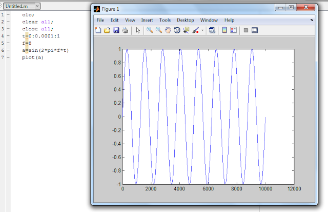
1) clc   (clear command window) :- syntax : clc description :- when user writes clc in program or in command window then the content of command window will be cleared. After using the clc user can not undo or get back the erased data of command window. 2)   clear all  :- syntax : clear all description :- when user writes clear all in program or in command window then the content of workspace will be cleared. After using the clear all user can not undo or get back the erased data of workspace. 3)   close all  :- syntax : close all description :- when user writes close all in program or in command window then the some window such as figure window will be closed. After using the close all user can not undo or get back the closed window. 4)   plot :- syntax : plot(a) description :- This command is used to plot some waves and some data. This command plot the data or wave in the x-y plane. Example:- 4)  sub plot :- syntax : subplot(r,c,p) description :

Different image operation (Addition, Subtraction, Multiplication, Division) of images using MATLAB

Image
1. Introduction :- In image processing many image operations are required including addition, subtraction, multiplication, division of images. 2 . Problem Statement :- To study different image operation. 3. Program :- clc; clear all; close all; a=imread('C:\Users\akshay\Pictures\desert.jpg'); subplot(3,2,1); imshow(a) title('1st input image') b=imread('C:\Users\akshay\Pictures\koala.jpg'); subplot(3,2,2); imshow(b) title('2nd input image') c=imadd(a,b); subplot(3,2,3); imshow(c) title('Addition of images') d=imsubtract(a,b); subplot(3,2,4); imshow(d) title('Subtraction of images') e=immultiply(a,b); subplot(3,2,5); imshow(e) title('Multiplication of images') f=imdivide(a,b); subplot(3,2,6); imshow(f) title('Division of images') 4. How to use this code :- Here you have to only copy the code to MATLAB and and give the location of the images on which you wants to perform given operation. 5.

Plot different window function using MATLAB

Image
1. Introduction :- Window function plays vital role in IIR filter designing. Hence while designing filter window is required. 2 . Problem Statement :- To plot different window using MATLAB. 3. Program :- clc; clear all; close all; l=64; a=bartlett(l); subplot(8,2,1); plot(a) title('bartlett window') b=barthannwin(l); subplot(8,2,2); plot(b) title('barthannwin window') c=blackman(l); subplot(8,2,3); plot(c) title('blackman window') d=blackmanharris(l); subplot(8,2,4); plot(d) title('blackmanharris window') e=bohmanwin(l); subplot(8,2,5); plot(e) title('bohmanwin window') f=chebwin(l); subplot(8,2,6); plot(f) title('chebwin window') g=flattopwin(l); subplot(8,2,7); plot(g) title('flattopwin window') j=hamming(l); subplot(8,2,8); plot(j) title('hamming window') k=hann(l); subplot(8,2,9); plot(k) title('hann window') m=kaiser(l); subplot(8,2,10); plot(m) title('kai

How to plot AM (Amplitude Modulated) signal using MATLAB

Image
1. Introduction :- AM wave is defined as the amplitude of carrier is varies with respect to the modulating signal. These signals are used in AM transmission and reception. 2 . Problem Statement :- To plot AM(Amplitude Modulated) signal using MATLAB. 3. Program :- clc; clear all; close all; t=0:0.0001:1; em=5; ec=5; fm=10; fc=100; a=em*sin(2*pi*fm*t); subplot(5,1,1); plot(t,a); xlabel('time'); ylabel('amplitude'); title('modulating signal'); b=ec*sin(2*pi*fc*t); subplot(5,1,2); plot(t,b); xlabel('time'); ylabel('amplitude'); title('carrier signal'); m=0.5 ec=em/m; c=ec*(1+m*sin(2*pi*fm*t)).*sin(2*pi*fc*t); subplot(5,1,3); plot(t,c) xlabel('time'); ylabel('amplitude'); title('under modulated signal'); m=1 ec=em/m; c=ec*(1+m*sin(2*pi*fm*t)).*sin(2*pi*fc*t); subplot(5,1,4); plot(t,c) xlabel('time'); ylabel('amplitude'); title('perfect modulated signal'

How to plot FM wave using MATLAB

Image
1. Introduction :- FM wave is defined as the frequency of carrier wave is varies with respect to the modulating signal. These signals are used in FM transmission and reception. 2 . Problem Statement :- To plot FM(Frequency Modulated) signal using MATLAB. 3. Program :- clc; clear all; close all; t=0:0.0001:1; em=5; ec=5; fm=10; fc=100; a=em*sin(2*pi*fm*t); subplot(3,1,1); plot(t,a); xlabel('time'); ylabel('amplitude'); title('modulating signal'); b=ec*sin(2*pi*fc*t); subplot(3,1,2); plot(t,b); xlabel('time'); ylabel('amplitude'); title('carrier signal'); m=1; c=ec*sin(2*pi*fc*t+m*a); subplot(3,1,3); plot(t,c) xlabel('time'); ylabel('amplitude'); title('modulated signal'); 4. How to use this code :- Here you have to only copy the code to MATLAB and just run it and on figure window all signal will appear. 5. Output  :-   Figure Window                                   6

How to find force using coulomb's law by using MATLAB.

Image
1. Introduction :- The coulomb's law states that like charges repel and opposite charges attracts with force which is proportional to the product of charges and inversely proportional to distance between them. 2 . Problem Statement :- To find magnitude using coulomb's law by using MATLAB. 3. Program :- clc; clear all; close all; q0=1e-9; q1=1; q2=1; p0=[2 0 0]; p1=[0 1 0]; p2=[0 -1 0]; eps=8.854e-12; r10=(sum((p0-p1).^2)).^(1/2); r20=(sum((p0-p2).^2)).^(1/2); r10u=(p0-p1)/r10; r20u=(p0-p2)/r20; f=q0*q1*r10u/(4*pi*eps*r10*r10)+q0*q2*r20u/(4*pi*eps*r20*r20); fmag=sqrt(sum(f.*f)); display (f) 4. How to use this code :- Here you have to only copy the code to MATLAB and just run it. 5. Output  :-   Figure Window                                   6. Conclusion  - Here we have   find force using coulomb's law by using MATLAB .

How to plot DFT (Discrete Fourier Transform) and IDFT (Inverse Discrete Fourier Transform) using MATLAB

Image
1. Introduction :- DFT is very important type of fourier transform which is use for fourier analysis in many application. It is used to determine frequency component in time domain signal. 2 . Problem Statement :- To find DFT using MALAB and plot phase spectrum and magnitude plot. 3. Program :- clc; clear all; close all; x=input('enter the sequemce') N=length(x); for n=0:N-1   for k=0:N-1     wnk(n+1,k+1)=exp(-i*2*pi.*n.*k/N);   end end dft=wnk*x'; display('dft of sequence is') display(dft) %plot original signal n=0:N-1; subplot(2,2,1) stem(n,x) xlabel('discrete time n') ylabel('amplitude') title('original signal') % magnitude plot k=0:N-1; subplot(2,2,2) stem(k,abs(dft)) xlabel('discrete frequency k') ylabel('amplitude') title('magnitude plot') % phase spectrume k=0:N-1; subplot(2,2,3) stem(k,angle(dft)) xlabel('discrete frequency k') ylabel('amplitude') title(&#